用户指南
在将这个发布于 PyPI 的开源库 PyPop7 应用于现实世界的黑盒优化(BBO)问题之前,应按顺序阅读以下四个基本信息:
问题定义
首先,需要以函数(function)的形式定义一个目标函数(在演化计算中也称为适应度函数,或在机器学习中称为损失函数)。然后,使用数据结构 dict 作为一种简单而有效的方式来存储与当前优化问题相关的所有设置,例如:
fitness_function:需要被最小化的目标/成本函数(func),
ndim_problem:问题的维度数量(int),
upper_boundary:搜索范围的上边界(array_like),
lower_boundary:搜索范围的下边界(array_like)。
不失一般性,本库只考虑最小化过程,因为最大化问题可以简单地通过对其目标函数取反来轻松转换为最小化问题。
下面是一个简单的例子,用于定义优化领域中众所周知的测试函数 Rosenbrock 函数:
1>>> import numpy as np  # engine for numerical computing
2>>> def rosenbrock(x):  # to define the fitness function to be minimized
3...     return 100.0*np.sum(np.square(x[1:] - np.square(x[:-1]))) + np.sum(np.square(x[:-1] - 1.0))
4>>> ndim_problem = 1000  # to define its settings
5>>> problem = {'fitness_function': rosenbrock,  # cost function to be minimized
6...            'ndim_problem': ndim_problem,  # dimension of cost function
7...            'lower_boundary': -10.0*np.ones((ndim_problem,)),  # lower search boundary
8...            'upper_boundary': 10.0*np.ones((ndim_problem,))}  # upper search boundary
当适应度函数本身除了采样点 x 之外还涉及其他输入参数时(这里我们区分输入参数和上述的问题设置),有两种简单的方法来支持这种更复杂的情况:
1) 创建一个类(class)包装器,例如:
 1>>> import numpy as np  # engine for numerical computing
 2>>> def rosenbrock(x, arg):  # to define the fitness function to be minimized
 3...     return arg*np.sum(np.square(x[1:] - np.square(x[:-1]))) + np.sum(np.square(x[:-1] - 1.0))
 4>>> class Rosenbrock(object):  # to build a class wrapper
 5...     def __init__(self, arg):  # arg is an extra input argument
 6...         self.arg = arg
 7...     def __call__(self, x):  # for fitness evaluations
 8...         return rosenbrock(x, self.arg)
 9>>> ndim_problem = 1000  # to define its settings
10>>> problem = {'fitness_function': Rosenbrock(100.0),  # cost function to be minimized
11...            'ndim_problem': ndim_problem,  # dimension of cost function
12...            'lower_boundary': -10.0*np.ones((ndim_problem,)),  # lower search boundary
13...            'upper_boundary': 10.0*np.ones((ndim_problem,))}  # upper search boundary
2) 利用本库为所有 BBO 提供的易于使用的统一(API)接口,例如:
 1>>> import numpy as np  # engine for numerical computing
 2>>> def rosenbrock(x, args):
 3...     return args*np.sum(np.square(x[1:] - np.square(x[:-1]))) + np.sum(np.square(x[:-1] - 1.0))
 4>>> ndim_problem = 10
 5>>> problem = {'fitness_function': rosenbrock,  # cost function to be minimized
 6...            'ndim_problem': ndim_problem,  # dimension of cost function
 7...            'lower_boundary': -5.0*np.ones((ndim_problem,)),  # lower search boundary
 8...            'upper_boundary': 5.0*np.ones((ndim_problem,))}  # upper search boundary
 9>>> from pypop7.optimizers.es.maes import MAES  # replaced by any other BBO in this library
10>>> options = {'fitness_threshold': 1e-10,  # to terminate when the best-so-far fitness is lower than 1e-10
11...            'max_function_evaluations': ndim_problem*10000,  # maximum of function evaluations
12...            'seed_rng': 0,  # seed of random number generation (which should be set for repeatability)
13...            'sigma': 3.0,  # initial global step-size of Gaussian search distribution
14...            'verbose': 500}  # to print verbose information every 500 generations
15>>> maes = MAES(problem, options)  # to initialize the black-box optimizer
16>>> results = maes.optimize(args=100.0)  # args as input arguments of fitness function
17>>> print(results['best_so_far_y'], results['n_function_evaluations'])
187.57e-11 15537
当除了采样点 x 之外还有多个(>=2)输入参数时,应通过函数或类包装器将它们组织起来(以dict或tuple的形式)。
高级用法
通常,upper_boundary 和 lower_boundary 这两个问题定义对于大多数终端用户来说已经足够控制初始搜索范围了。然而,有时出于优化器基准测试的目的(例如,为了避免利用对称性和原点可能带来的搜索偏见),我们增加了两个额外的定义来控制种群/个体的初始化:
initial_upper_boundary:仅用于初始化的上边界(array_like),
initial_lower_boundary:仅用于初始化的下边界(array_like)。
如果没有明确给出,initial_upper_boundary 和 initial_lower_boundary 将分别被设置为 upper_boundary 和 lower_boundary。当明确给出 initial_upper_boundary 和 initial_lower_boundary 时,种群/个体的初始化将从 [initial_lower_boundary, initial_upper_boundary] 而不是 [lower_boundary, upper_boundary] 中采样。
优化器设置
本库为所有 BBO 的超参数设置提供了一个统一的 API。以下算法选项(都存储在字典(dict)格式中)对于所有 BBO 都非常常见:
max_function_evaluations:函数评估的最大次数(int,默认值:np.inf),
max_runtime:允许的最大运行时间(float,默认值:np.inf),
seed_rng:需要被明确设置的随机数生成(RNG)种子(int)。
应根据可用的计算资源或可接受的运行时间(即,与问题相关),至少设置 max_function_evaluations 和 max_runtime 这两个算法选项中的一个。为了可复现性,应为随机数生成(RNG)明确设置 seed_rng。请注意,由于不同的 NumPy 版本可能使用不同的 RNG 实现,可复现性主要在同一 NumPy 版本内得到保证。
请注意,对于任何优化器,其特定的选项/设置(详见其 API 文档)可以很自然地添加到 dict 数据结构中。以著名的交叉熵方法(CEM)为例。其高斯采样分布的均值和标准差的设置通常对收敛速度有显著影响(有关其超参数的更多详细信息,请参阅其 API):
 1>>> import numpy as np
 2>>> from pypop7.benchmarks.base_functions import rosenbrock  # function to be minimized
 3>>> from pypop7.optimizers.cem.scem import SCEM
 4>>> problem = {'fitness_function': rosenbrock,  # define problem arguments
 5...            'ndim_problem': 10,
 6...            'lower_boundary': -5.0*np.ones((10,)),
 7...            'upper_boundary': 5.0*np.ones((10,))}
 8>>> options = {'max_function_evaluations': 1000000,  # set optimizer options
 9...            'seed_rng': 2022,
10...            'mean': 4.0*np.ones((10,)),  # initial mean of Gaussian search distribution
11...            'sigma': 3.0}  # initial std (aka global step-size) of Gaussian search distribution
12>>> scem = SCEM(problem, options)  # initialize the optimizer class
13>>> results = scem.optimize()  # run the optimization process
14>>> # return the number of function evaluations and best-so-far fitness
15>>> print(f"SCEM: {results['n_function_evaluations']}, {results['best_so_far_y']}")
16SCEM: 1000000, 10.328016143160333
结果分析
优化阶段结束后,所有黑盒优化器都会以一种统一的方式返回至少以下常见结果(收集到一个字典(dict)数据结构中):
best_so_far_x:优化过程中找到的迄今为止最优的解,
best_so_far_y:优化过程中找到的迄今为止最优的适应度(即目标值),
n_function_evaluations:优化过程中使用的函数评估总次数(永远不会超过 max_function_evaluations),
runtime:整个优化阶段使用的总运行时间(不会超过 max_runtime),
termination_signal:来自三个常见候选项(MAX_FUNCTION_EVALUATIONS、MAX_RUNTIME 和 FITNESS_THRESHOLD)的终止信号,
time_function_evaluations:仅在函数评估中花费的总运行时间,
fitness:在整个优化阶段生成的适应度(即目标值)列表。
当优化器选项 saving_fitness 设置为 False 时,fitness 将为 None。当优化器选项 saving_fitness 设置为整数 n (> 0) 时,fitness 将是每 n 次函数评估生成一次的适应度列表。请注意,第一个和最后一个适应度值总是作为优化的开始和结束而被保存。在实践中,适当地设置 saving_fitness 可以为最终的优化结果生成一个低内存的数据存储。
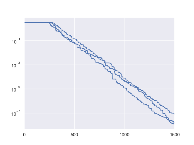
下面是一个简单的例子,用于可视化 Rechenberg 的 (1+1)-演化策略在经典 sphere 函数(最简单的测试函数之一)上的适应度收敛过程:
 1>>> import numpy as np  # https://link.springer.com/chapter/10.1007%2F978-3-662-43505-2_44
 2>>> import seaborn as sns
 3>>> import matplotlib.pyplot as plt
 4>>> from pypop7.benchmarks.base_functions import sphere
 5>>> from pypop7.optimizers.es.res import RES
 6>>> sns.set_theme(style='darkgrid')
 7>>> plt.figure()
 8>>> for i in range(3):
 9>>>     problem = {'fitness_function': sphere,
10...                'ndim_problem': 10}
11...     options = {'max_function_evaluations': 1500,
12...                'seed_rng': i,
13...                'saving_fitness': 1,
14...                'x': np.ones((10,)),
15...                'sigma': 1e-9,
16...                'lr_sigma': 1.0/(1.0 + 10.0/3.0),
17...                'is_restart': False}
18...     res = RES(problem, options)
19...     fitness = res.optimize()['fitness']
20...     plt.plot(fitness[:, 0], np.sqrt(fitness[:, 1]), 'b')  # sqrt for distance
21...     plt.xticks([0, 500, 1000, 1500])
22...     plt.xlim([0, 1500])
23...     plt.yticks([1e-9, 1e-6, 1e-3, 1e0])
24...     plt.yscale('log')
25>>> plt.show()
高级用法
根据一位最终用户最近的建议,我们添加了 EARLY_STOPPING 作为第四种终止信号。详情请参考 #issues/175。
算法选择与配置
对于大多数现实世界的黑盒优化问题,通常几乎没有先验知识可以作为算法选择的基础。也许最简单的算法选择方法是试错法。然而,我们仍然希望在此提供一个经验法则,以根据算法分类来指导算法选择。有关三种不同分类族(仅基于维度)的详细信息,请参阅我们的 GitHub 主页。值得注意的是,这种分类仅仅是对算法选择的一个非常粗略的估计。在实践中,算法的选择主要应取决于关注的性能标准(例如,收敛速度和最终解的质量)以及可用的最大运行时间。
未来,我们期望将自动化算法选择与配置技术加入到这个开源 Python 库中,如下所示(仅举几例):
Lindauer, M., Eggensperger, K., Feurer, M., Biedenkapp, A., Deng, D., Benjamins, C., Ruhkopf, T., Sass, R. and Hutter, F., 2022. SMAC3:一个用于超参数优化的通用贝叶斯优化包。JMLR, 23(54), pp.1-9。
Schede, E., Brandt, J., Tornede, A., Wever, M., Bengs, V., Hüllermeier, E. and Tierney, K., 2022. 自动化算法配置方法综述。JAIR, 75, pp.425-487。
Kerschke, P., Hoos, H.H., Neumann, F. and Trautmann, H., 2019. 自动化算法选择:综述与展望。ECJ, 27(1), pp.3-45。
Probst, P., Boulesteix, A.L. and Bischl, B., 2019. 可调性:机器学习算法超参数的重要性。JMLR, 20(1), pp.1934-1965。
Hoos, H.H., Neumann, F. and Trautmann, H., 2017. 自动化算法选择与配置(Dagstuhl 研讨会 16412)。Dagstuhl Reports, 6(10), pp.33-74。
Rice, J.R., 1976. 算法选择问题。In Advances in Computers (Vol. 15, pp. 65-118). Elsevier。